Average Doesn't Always Exist
Up until now, I thought average always exists. We are dealing with average very often in real life: the average height of Japanese, the average rate of divorcing in US, and the average salary in France, etc. It seemed to me that if I take enough number of sample data, I can get average that reflects the reality very well.
Today I learned that this is not always the case. Average doesn’t always exist. Because the idea is very interesting to me, let me share the idea with you.
Average in Coin Toss Game
Let’s being with the case when average exists. I’ll use a very simple coin toss game. You flip a coin and you win $1 if the result is head. You win $0 or nothing if the result is tail. Very simple.
When you toss the coin multiple times, what’s the average of dollar you will win? You can get the average very easily by the following formula:
avg. = (total number of $ you won) / number of times you toss the coin
And you will see that the average is 0.5 because the chance of getting head is 1/2. But is it really so? Let’s confirm this by writing some code to simulate the game.
Here is a small Clojure code to simulate the game.
(defn toss-coin []
  (rand-int 2))

(defn do-coin-toss [ite]
  (loop [n 1 total 0 avg []]
    (if (> n ite)
      (map float avg)
      (do
        (let [outcome (toss-coin)]
          (recur (+ n 1) (+ total outcome) (conj avg (/ total n))))))))

(defn write-data [col]
  (let [vec (map-indexed (fn [idx item]
                           (str idx " " item)) col)
        data (clojure.string/join "\n" vec)
        header "n avg\n"
        file "/tmp/coin-toss-result.txt"]
    (spit file header)
    (spit file data :append true)
    (spit file "\n" :append true)))
Here is R program draw.R to draw a graph.
ind = commandArgs(trailingOnly=TRUE)[1]
file = "coin-toss.png"

(x <- read.table("/tmp/coin-toss-result.txt", header=T))
png(file)
plot(x$avg, type="l")
dev.off()
browseURL(file)
If you want to toss the coin 10 times and output the result to a text file, you can do (write-data (do-coin-toss 10)) from REPL and run
Rscript draw.R
``` from your terminal.
I'll denote n as the number of times you toss the coin for brevity from now on.
Here is the graph of the average when n is **10**.
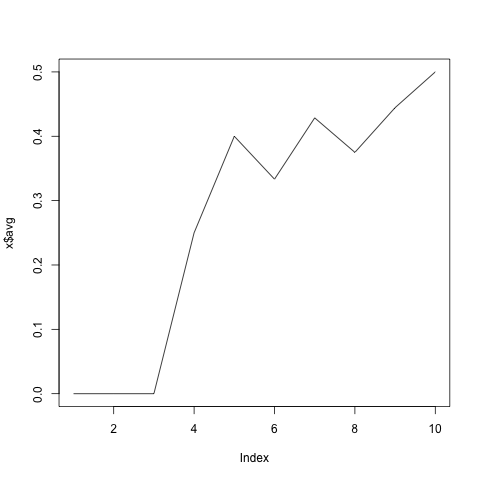
As you can see, the average is very quickly approaching to **0.5**. Let's do the same thing with larger n.
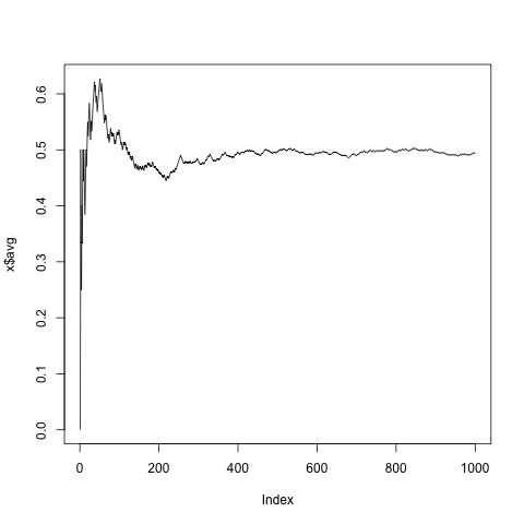
When n is **1000**
When n is **10000**
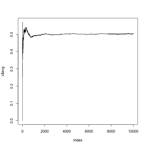
By looking at these graphs, we can safely say that the average of dollar you win in this coin toss game is $0.5.
## When Average Doesn't Exist.
Now we are entering an interesting area where the average disappears. To illustrate this, we will make the coin toss game a bit more complicated.
This time, you keep flipping the coin until you get head and you will get **2 ^ (number of times you flip the coin)**.
For example, if your result is tail, tail, and then head, then you get **2 ^ 3** (because you flipped three times) which is $8. Let's call this game "coin-toss-unti-head" game.
Here is a Clojure code to simulate the coin-toss-until-head game.
```clojure
(defn exp [x n]
(if (zero? n) 1
(* x (exp x (dec n)))))
(defn toss-coin-until-head []
(loop [n 1]
(let [outcome (toss-coin)]
(if (= 0 (toss-coin))
(exp 2 n)
(recur (+ n 1))))))
(defn do-coin-toss [ite]
(loop [n 1 total 0 avg []]
(if (> n ite)
(map float avg)
(do
(let [outcome (toss-coin)]
(recur (+ n 1) (+ total outcome) (conj avg (/ total n))))))))
(defn write-data [col]
(let [vec (map-indexed (fn [idx item]
(str idx " " item)) col)
data (clojure.string/join "\n" vec)
header "n avg\n"
file "/tmp/coin-toss-result.txt"]
(spit file header)
(spit file data :append true)
(spit file "\n" :append true)))
You can again run the code from REPL
(write-data (do-coin-toss 10 toss-coin-until-head))
and plot graphs with
Rscript draw.R
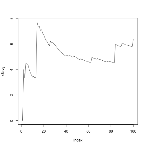
Let’s begin with n=10.
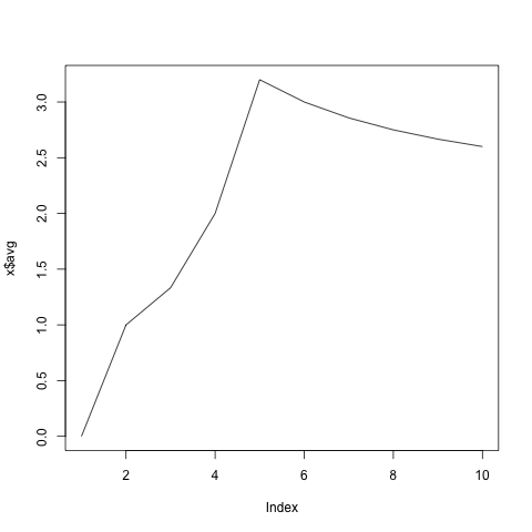
It looks like the average is approaching to somewhere around 2.5 but we are not fully sure yet. Let’s increase n and see if the average is really 2.5.
Here is the graph when n is 20 and you will probably be disappointed by looking at the graph: the average is approaching to 2.5 and then suddenly there is a spike around n=20 which pushes the average a way higher! You will also discover the pattern after n=20: the average is converging to a number but then you will see a spike shortly after the convergence.
Maybe we just haven’t tossed the coin enough times. Let’s keep going a bit further.
Here is the graph when n is 10000. It looks like this time the average is approaching to somewhere around 12. Did we finally discover the average?
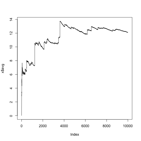
It turns out we didn’t! This is very clear when you increase n to 50000.
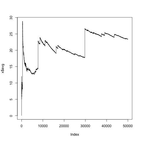
Again, there is a spike around 30000 and we lost the average again. You can increase n as much as you want and you will never find a good average in this game.
Why Average Doesn’t Exist?
We can see why the average doesn’t exist with simple math.
You can calculate the average of normal coin-toss game with the following formula.
ave. = (probability of H) x $1 + (probably of T) x $0
Because both the probability of getting head (H) and tail (T) is 0.5, the average of dollar you will win becomes $0.5 which is what we’ve seen in the previous simulations.
Let’s compute the average for the coin-toss-until-head game. One big difference from the normal coin toss game is that there are infinite numbers of different results of coin in this game. The result could be T H or T T H or T T T T T T H or whatever.
So we need to calculate all the possibilities. You can express this with the following formula.
ave. = (probability of H) x 2^1 + (probability of TH) x 2^2 + (probably of TTH) x 2^3 ......
When you plugin the actual probability to the formula above, this will become the following.
ave. = (1/2) x 2^1 + (1/2 x 1/2) x 2^2 + (1/2 x 1/2 x 1/2) x 2^3 ......
ave. = 1 + 1 + 1 ......
ave. = ∞ (infinity)
The average that you got is ∞ (infinity). In other words, average doesn’t exist.
What’s the implication of the idea that average doesn’t always exist in real life?
Another way of interpreting these graphs without average is that sometimes a super extreme event could happen. Because the impact of the event is astronomical, it skews the average and make it useless. So, if the model that you are studying is similar to the coin-toss-until-head game, you will see the same pattern. In fact, this model is often used to study extreme events such as a sudden collapse in a stock market.
Summary
Hopefully, you will find this interesting. Time is running out, so I’ll stop here, but if you want to learn more, you can search “St. Petersburg paradox” or “Power Laws” to dive into the area deeper.
You can find code I used here at https://github.com/kimh/coin-toss